In “Graphs at Work” I claim

To improve the customer experience, what you need to understand is the distribution of strategy performances for a given algorithm on real-world graphs, not the theoretical worst case.

Of course, that’s a simplification. Theoretical worst-case performance does impact the customer experience, either on accident or because some adversary wants to throttle your program. Worry less if your “customer concerns are well-isolated,” but they rarely are.

By “real-world graphs” I suggested a family of associations graphs, distinct from the family of all possible associations graphs, might describe the bulk of customer desires. For example, if the typical customer associates Contacts, Deals, and other objects via a mutual association with a Company, those customers’ “real-world graphs” will approximate stars with the Company at the center.

Parameterizing those graph families, you can simulate the candidate algorithms’ performance against a wide range of possible customer configurations (even configurations impossible in practice, e.g. because of a limit on the number of HubSpot types).

Experiment space

All the uncertainty about what’s “real-world” translates into a huge experimental space. Any given experiment embeds a set of assumptions about what the user probably wants and what they have in HubSpot. All the experiments taken together are only useful if they describe the problem well enough, in all its dimensions, to react to user information as it comes in.

Most of the variables here are discrete categories — different vertex cover algorithms, different topological families of graphs, and different weighting schemes for vertices. For these purposes, there isn’t a continuous space between Vazirani’s algorithm and Lavrov’s.

Some of those categories introduce scalar variables, like the size of a random graph or the probability two vertices are adjacent.

Vertex cover algorithms

An unweighted vertex cover algorithm will never k-approximate a minimal weighted vertex cover. Unweighted algorithms behave as if all vertices have the same weight, then minimize the number of vertices in the cover V_req. When you add weights to G = {V, E}, V_req might be arbitrarily bad: each vertex in V_req can be arbitrarily expensive, and vertices in V − V_req can be arbitrarily cheap.

Obviously the best an unweighted algorithm can perform on a weighted graph is to accidentally suggest the weighted optimal strategy.

How should we expect it to perform given a random distribution of weights? I think of a single graph with its topology-determined minimum unweighted vertex cover V_req. The expected weight of that vertex cover is μ∥V_req∥ where μ is the mean of the weight distribution.

What if weights aren’t distributed randomly, and instead correlate with graph topology? I’m not sure what to expect. That question is easier to simulate than to theorize.

I implement three of the algorithms discussed in my last post.

clever

The greedy algorithm I previously implemented in Elixir. I came up with it independently, but I take the name from Michel Zito.¹

The punchline: this algorithm isn’t clever. It performs so badly on tricky graphs it doesn’t k-approximate minimal vertex covers. To this algorithm’s credit, it has an intuitive heuristic: add the highest-degree vertex in G to V_req, remove it from G, and recurse for a minimal vertex cover on what remains.

lavrov

the “2-approximating [unweighted] vertex cover” variation suggested by Mikhail Lavrov:

Start with V_req = ∅. Then, as long as V_req doesn’t cover every edge, we pick an uncovered edge and add both endpoints to V_req.²

My implementation is an even greedier variant, at the cost of some runtime complexity: rather than arbitrarily picking an uncovered edge, it picks the uncovered edge with the highest combined degree between its incident vertices. Lavrov proves the 2-approximation.

vazirani

The only weighted vertex cover algorithm I implement. Rather than removing vertices outright, it relaxes virtual weights t(v) for the vertices incident on a “taken” (uncovered) edge, then adds one or both to V_req depending on the result. My implementation leaves edge-selection arbitrary, per Vazirani’s definition.³

As the only k-approximation of a minimum weighted vertex cover, it’s safe to assume vazirani should perform the most stably. That doens’t moot the experiment. As I noted, there are graphs where it yields a worse result than clever!

Topologies

Well, what’s a “real-world graph?” In the absence of customer data — I don’t have any — we can try simulating several parameterized families of graphs instead of just guessing. I implement two families.

random

A graph with n vertices. Any pair v₁, v₂ ∈ V are connected with probability p. Notably, these graphs have a nondeterministic total connectivity — there’s always a p²ⁿ chance of getting a complete graph! — but that’s just a reason to simulate repeatedly.

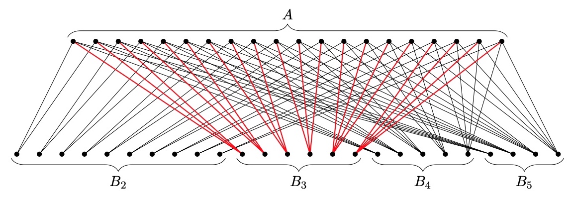
tricky

“Tricky” graphs follow a construction from Lavrov designed to force the clever algorithm into arbitrarily bad vertex covers. Instead of taking a number of vertices, the construction starts with integers a and k ≤ a; then

On one side of the graph, put n vertices, for some (large) n. Call the set of these vertices A.

On the other side of the graph, put k − 1 “blocks” of vertices, numbered B₂, B₃, ..., B_k. Block B_i will have ⌊n/i⌋ vertices.

Each vertex in A gets one edge to a vertex in B_i, and they are distributed as evenly as possible: each vertex in B_i ends up with either i or i + 1 neighbors in A.⁴

What makes it tricky? Initially the highest-degree vertices are in B_k. When clever has included those in the cover V_req, the highest-degree vertices are in B_k − 1. This continues until V_req = B₂ ∪ B₃ ∪ ... ∪ B_k, even though there’s a smaller vertex cover staring right at us: A!

These graphs have a ⋅ H_k vertices, where H_k is the kth harmonic number: ∥A∥ = a and ∥B_i∥ = (i^− 1)a.

There are potentially many more families to explore. Like I mention above, stars might capture HubSpot’s ontology for built-in types well: it’s a CRM, so pretty much everything associates, directly or indirectly, with a Company. Graphs composed of stars, joined at the leaves, might reflect HubSpot customers using custom objects to hang subontologies off of the built-in types: a Company’s association with a Deal indirectly associates it with a collection of Deal-specific custom object types.

I considered testing a “small-world” family of graphs, with vertices highly-adjacent to “neighbors” and adjacent to non-“neighbors” with some lower probability, but I’m not sure it’s relevant to the HubSpot problem definition. There’s no natural concept of “neghbors” among HubSpot object types. Remember: customer “configurations” are subgraphs of a complete graph of types. Emergent graphs — especially physical networks — may well have small-world properties, but it’s less clear why a subtractive configuration-selection process would yield them.

Weight schemes

The cost of requesting the objects of a HubSpot type is the number of members divided by the APIs request page size. How many objects of each type exist? Who knows! Like with graph families, it’s easier to simulate several of them than to evidence-free agonize over which is “realest.”

uniform

Assigns every vertex the same weight, unweighting the vertex cover problem.

random

Assigns each vertex a random weight on the half-open interval [0, 1).

degree-negative

A weight scheme where a vertex’s weight is negatively correlated with its degree. To keep weights positive, I use (d(v) + ϵ)^− 1, where ϵ is a small positive constant to prevent divison-by-zero panics on disconnected vertices.

degree-positive

Each vertex’s weight is its degree.

degree-positive-superlinear

Each vertex’s weight is the square of its degree.

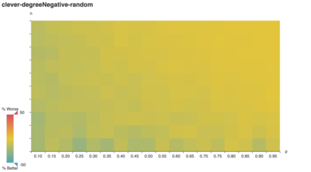
I expect degree-negative and degree-positive to reward and punish the clever algorithm, respectively. clever gobbles high-degree vertices into V_req oblivious to their weight. In one case that greedy strategy correlates with low weights, in the other case with high.

Project structure

Why reach for Go? My first instict was to use built-in benchmarking to compare algorithms. That is a cool tool (one of my favorite take-home interview hacks) but I don’t wind up using it. Runtime performance is just too dependent on implementation details; I’m better off spending my time building a graph package with a decent interface than, say, using separate graph implementations optimized for each algorithm.

There are other, better reasons to write Go. Static types prevent a suite of bugs I’d encounter in Python — Go’s a “when it compiles, it does what you mean” experience — and module management is simpler than in Typescript. The standard testing library is pleasant. godoc is built in, and linters abound.

The stand-out advantage, I found, is a convention: the standard Go project layout, which separates reusable library code in pkg subdirectories from applications in cmd, is well-suited to experimentation. I wound up with a project structure like this:

The simulation models depend on one another, but they’re independent of the experiments that use them. pkg/graph exports weighted and unweighted graphs, along with some known graphs used in tests. pkg/cover implements vertex cover algorithms on those graph types.

Both packages include tests. Testing is especially useful in pkg/cover, where it tests two kinds of correctness: that my code behaves how I expect it to, and that my expectations match the algorithm definitions in literature! By testing on known graphs (defined in pkg/graph/fixtures.go), I check my implementations match examples from papers. TestClever_Tricky confirms clever selects V_req = B like Lavrov claims; if it doesn’t, there’s some mistake in the implementation even if it yields valid vertex covers.

Experiments go in subdirectories of cmd. Each directory is space for notes, outputs, experiment-specific helper code, and so on. Because there’s no risk of one experiment impacting the others — there aren’t interdependencies in cmd — these are scratchpads.

In summary:

1. Put reusable simulation components in pkg.
2. Use unit tests to confirm your implementations against prior art examples.
3. Explore in cmd.

Next time I might reach for a scientific computing package like Gonum to aggregate data in experiments. It even ships with a graph package, albeit one suited for edge-weighted problems over vertex-weighted ones.⁵

Simulations

Any pair of experiments should be comparable at a glance. Absolute vertex cover weights are sensitive to graph topology and individual vertex weights, which makes it hard to compare an algorithm’s performance on a ten-vertex graph against another algorithm’s performance on a hundred-vertex graph.

Instead, since my goal is to compare algorithms, I measure relative cover weight against a baseline: vazirani. Because it’s a 2-approximation, it guarantees a bound on any algorithm’s relative performance: if it’s implemented correctly, nothing can do more than 50% better than vazirani.

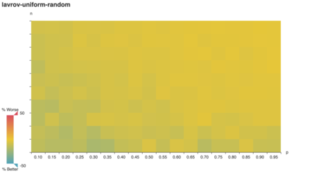
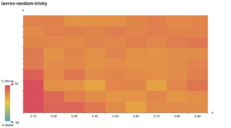
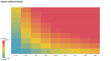
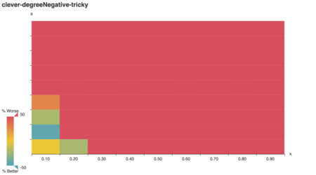
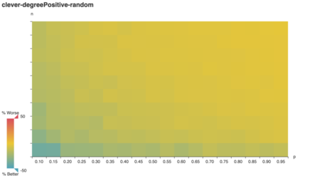
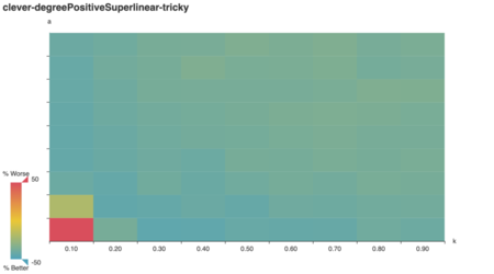
In the heatmaps below,

• -50 (teal) denotes a vertex weight 50% better than vazirani on the same graph.
• 0 (yellow) denotes a vertex weight at parity with vazirani.
• 50 (red) denotes a vertex weight 50% worse than vazirani. Worse performances are the same deep red — without a k-approximation, an algorithm can be worse up to the total weight of V!

Each cell averages ten relative performances: ten times, the simulation generates a graph G with the given parameters, then finds vertex covers on that G with the vazirani and tested algorithms.

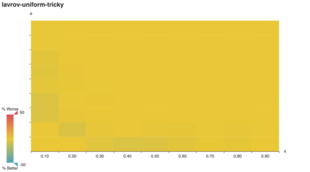
For starters, we can visually confirm a behavior predicted in literature: Lavrov’s tricky graphs are designed to arbitrarily damage the clever algorithm’s performance.

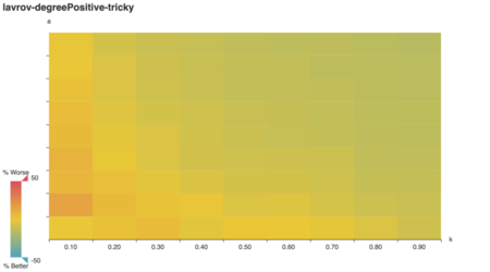
As Lavrov suggests, the “clever” algorithm is tricked for large a, k. (Note: while k is an integer in Lavrov’s tricky graph construction, here it’s expressed as a multiple of the number of vertices in A.) Does the lavrov algorithm do better?

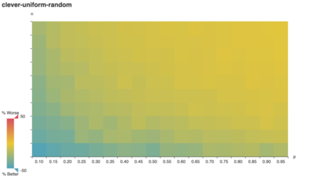
Indeed it does! Strikingly, lavrov performs just as well as vazirani on a uniformly-weigted graph. Upon reflection, I realize vazirani and lavrov are equivalent in a uniformly-weighted context: t(v) always goes to zero for u and v at every step, because both have the same starting weight!

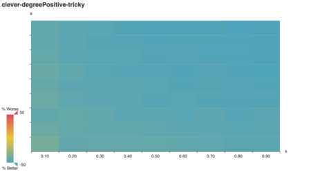
To my surprise, clever outperformed vazirani on tricky graphs when vertex weights corresponded 1:1 to degree.

On reflection, this makes sense too. Any vertex cover of a degree-positive-weighted graph covers every edge, which means it has a minimum weight ∥E∥. By minimizing redundant coverage, clever approximates that optimal cover. Since vazirani is a 2-approximation, the optimal cover is at most 50% better.

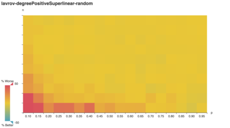
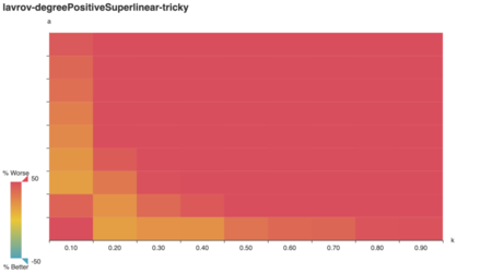
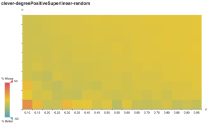
What if vertex weights are superlinearly positively correlated with vertex degree?

Huh! To my surprise, except for a low-n low-k blip, clever still generally outperforms vazirani. Even weirder:

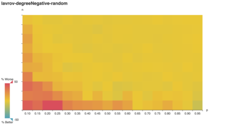
I expected degree-negative weighting would reward the clever algorithm for picking high-degree vertices, but it doesn’t!

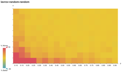
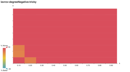
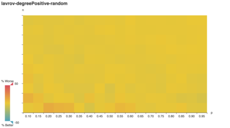
lavrov overview

A weight-naïve version of vazirani, lavrov achieves parity when it isn’t punished for weight-naïveté (when weights are uniform). Otherwise, vazirani’s performance lower-bounds it; you’d only prefer lavrov if you need its programmatic simplicity.

Weight/Topology	random	tricky
uniform
random
degree-negative
degree-positive
degree-positive-superlinear

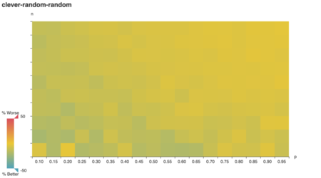
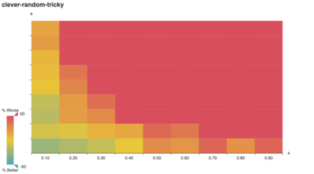
clever overview

As expected, clever does poorly on tricky graphs with uniform and random vertex weights.

Unexpectedly, it performs quite well on tricky graphs where vertex weight correlates positively with vertex degree! In domain-specific terms, that suggests clever is good choice if your HubSpot account’s most-associated types are also your most numerous collections.

I still gut-distrust this conclusion. It’s just so easy to think up a small but plausible associations graph where clever’s dismal because, say, you have hundreds of thousands of Contacts.

Weight/Topology	random	tricky
uniform
random
degree-negative
degree-positive
degree-positive-superlinear

If you want to poke around the experimental results, check out the full set of interactive graphs. If you want to reproduce them or inspect my implementations, see the source code on GitHub.